the-long-road-to-melody(7)
NAME
The Long Road To Melody Debugging autoregressive sequence models through Bach chorale generation.
FILED
DESCRIPTION
In 2022 I took a machine learning course that offered a handful of project options. One of them was Bach chorale generation: given a text file of four-part harmonies, train a model to continue a chorale in the style of Bach. The dataset was small, the format was simple, and polyphonic music generation seemed like a more honest test of sequence modeling than the usual toy problems. I had just started learning about recurrent models and how they work, so I chose this project.
The model we built produced output that fit the training distribution. The note ranges were right. The voice spacing looked plausible on paper. But played back as audio, it was noise. Notes jumped across octaves without direction. Voices moved in lockstep or collapsed into silence. The model had learned the statistics of Bach but none of the structure.
That failure stuck with me. Not because I expected a course project to produce beautiful music, but because the gap between “mathematically correct” and “sounds like music” exposed something worth understanding. Autoregressive models are prone to mode collapse, error accumulation, and outputs that drift into degenerate states over long sequences. Music makes these failures immediately audible in a way that a perplexity score on a language benchmark does not. You can hear when the model loses the thread.
This repo picks up where that project left off. The goal is not to build a practical music generation tool or to produce polished compositions. It is to treat the Bach chorale task as a controlled testbed for studying autoregressive models. What representations help a model stay coherent over long sequences? How much architectural complexity do you actually need? At what point does the output cross the threshold from statistical mimicry into something that sounds intentional?
I started with an LSTM because it was fast to iterate locally (16 hidden units, small enough to train on a laptop between experiments). I added a Transformer later to see whether self-attention changed the failure modes. There is also a linear regression baseline because if a linear model gets close, the problem is not as hard as you think. The end goal is to find the smallest possible model that produces melodic output, and then run ablation experiments to understand which components actually matter.
The problem
The dataset is a single text file: roughly 3,800 timesteps of Bach chorales, four columns for soprano, alto, tenor, and bass. Each value is a MIDI note number. Zero means silence. That is the entire input.
This looks straightforward, but it is not. There are four voices moving simultaneously with interdependent relationships. A chord sounds right or wrong because of the intervals between voices, not the absolute pitches. The model has to track counterpoint across four parallel streams while respecting the range and role of each voice. A single bad note in one voice cascades into the other three because the next prediction conditions on the full four-voice context.
The first obstacle is silence. Chorales begin with rests. The training data has long stretches of zeros at the start of every piece. A model optimizing for categorical cross-entropy quickly discovers that predicting silence is a low-risk strategy: zeros are common, easy to predict, and bring the loss down. I had to throw away the early windows during training to prevent the model from learning to output nothing. Even with that fix, the autoregressive generation loop remains vulnerable. If the model outputs a few zeros during generation, it has pushed itself into a region of the input space it never saw during training. Recovery from there is nearly impossible. The output stays silent forever.
Beyond silence, the failure modes are immediately audible. The model repeats the same two-bar phrase in an endless loop. Voices drift toward each other and collapse into unison, erasing the four-part texture. A note that is off by one semitone in the model’s output feeds back into the next prediction and pushes the whole sequence into harmonic territory that makes no sense. These are the classic symptoms of autoregressive degradation: small errors compound, the distribution shifts away from the training manifold, and the output spirals.
The original course project hit every one of these failures. We used PyTorch and trained four separate LSTM models, one per voice, each predicting its own note distribution independently. The models had no way to coordinate. The first working pipeline produced nothing but zeros. A later version produced notes but the durations were wrong: every note lasted exactly one timestep, giving the output a staccato, mechanical quality with no phrasing. When we varied the context window size, the output probabilities did not change. The model had collapsed to a fixed distribution that ignored its input. We tried a grid search to tune hyperparameters and it froze because the machine ran out of memory. One team member could not run the LSTM at all due to a runtime error we never resolved. The data representation was broken for weeks and we only knew because the output sounded wrong, not because any test failed.
Compounding all of this is the fact that bugs in a music generation pipeline are silent. The model trains. The loss decreases. TensorBoard looks fine. But the output is garbage, and you cannot tell from the metrics. When I returned to this project years later, I hit two more of these bugs that are worth describing because they illustrate how fragile the data pipeline remains even when you know what to look for.
The first was an integer overflow in the input encoding. The raw note
values were loaded as numpy.int8. When I computed the position of each
note on the circle of fifths, the expression 7 * note overflowed the
int8 range past note value 18, silently wrapping to a negative number.
The encoding was corrupted, but no exception was raised. The model
trained on garbage features and produced garbage output, and the loss
curve gave no indication anything was wrong.
The second was in the NoteSampler, a post-processing step that selects
the best candidate from the model’s output by scoring chord quality
against a distribution learned from Bach. The chord quality table is a
3D array indexed by the three intervals between four voices. For months,
the code indexed it with the four raw note values instead. The lookup
returned whatever happened to be at those out-of-bounds coordinates. The
scoring step was selecting candidates at random while reporting improved
metrics. One line fixed it: np.diff(notes) to compute the three
intervals before indexing.
These bugs share a common thread: in music generation, correctness is perceptual, not numerical. A language model with corrupted embeddings would produce nonsense tokens and a spike in perplexity. A music model with corrupted encodings produces notes that are still in range, still at plausible frequencies, still look fine on paper. You cannot debug it by watching the loss. You have to listen.
Underneath all of this is the representation problem. Raw MIDI note numbers carry no musical structure. Note 60 and note 61 differ by one integer, but note 60 and note 72 (an octave higher) differ by twelve. The model has to learn octave equivalence from scratch. It has to discover that certain intervals are consonant and others are not. It has to figure out voice ranges from data alone. With a dataset this small and a model this constrained, it will not learn these things on its own. The representation largely determines the ceiling.
How it works
The group project left off in early 2023 with a PyTorch pipeline that trained four independent LSTMs in a Jupyter notebook. It had the beginnings of the right ideas: the five-dimensional note encoding (chromatic circle, circle of fifths, log-scaled pitch, voice offset), a basic frequency-based sampler, and a rudimentary MIDI export. But the models did not share information across voices. The notebook had hardcoded paths and magic numbers. The data representation had shape bugs that took weeks to notice because nothing crashed, the output just sounded wrong. There was no way to run it from the command line or compare different configurations.
I rebuilt the pipeline from the ground up with a few deliberate choices.
Unified model. Instead of four separate LSTMs, a single model
predicts all four voices at once. The input is a window of shape
(timesteps, voices, features). The output is a softmax over all
possible notes for each voice simultaneously. This lets the model learn
the relationships between voices directly from the gradients rather than
hoping four independently trained models converge to something coherent.
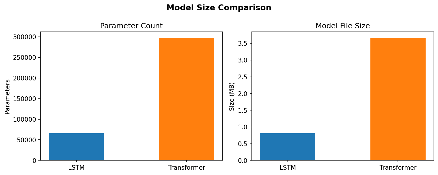
Two architectures. The LSTM model uses a Conv3D layer as a frontend to capture local patterns across time and voices, followed by a small LSTM (16 hidden units) and two dense layers. The Transformer model uses positional encoding and four self-attention blocks with 4 heads each, followed by global average pooling and a two-layer prediction head. Both models share the same data pipeline, the same Config interface, and the same generation loop, so they can be compared directly.
The LSTM was chosen first because it is simple and fast. With 16 hidden units it trains in seconds on a laptop, which matters when you are iterating on the data pipeline, the sampler logic, and the encoding. The Transformer was added later to see whether self-attention handles long-range dependencies differently. Right now the LSTM produces consistent output while the Transformer has a tendency toward long silences. More tuning is needed.
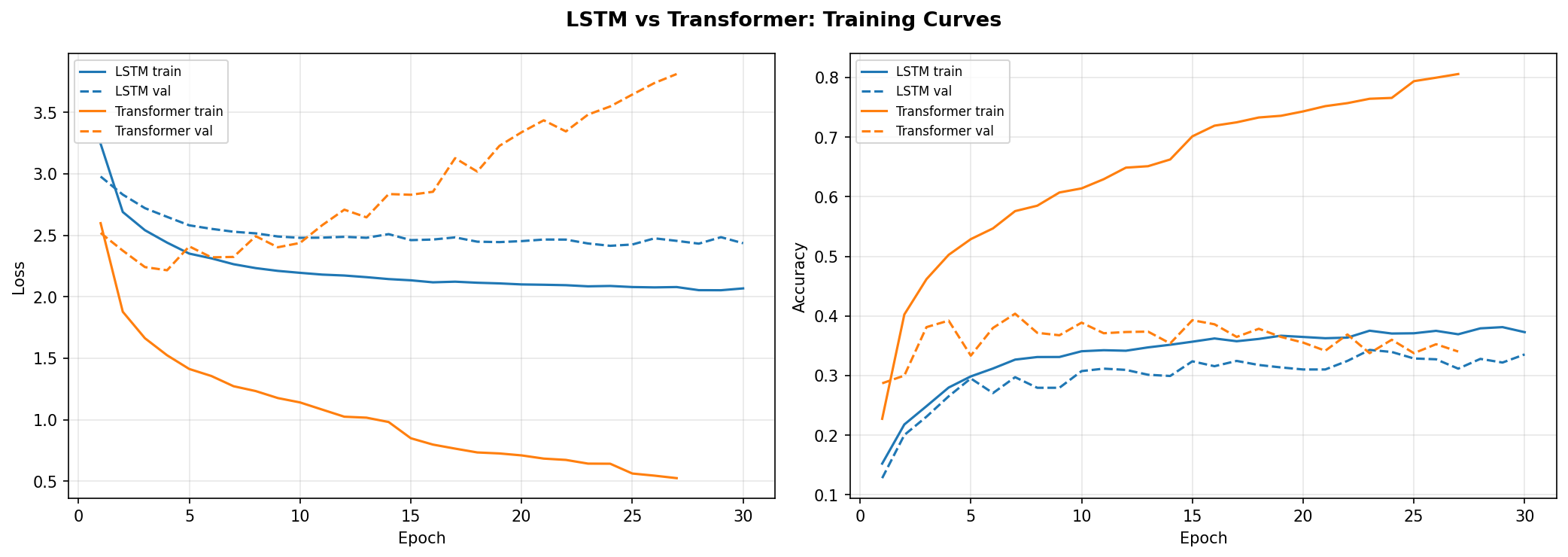
The training curves show the LSTM converging smoothly while the Transformer oscillates and its validation loss trends upward, a clear sign of overfitting on the limited dataset. The Transformer is new to the project and not yet optimized. It currently suffers from the same failure modes the early LSTM did: long silences and repetitive loops. More tuning is needed before it can be compared fairly.
Linear regression baseline. Before assuming any deep learning is necessary, I trained a Ridge regression model on the same windowed input. It fits a linear mapping from the encoded features to the note distribution and achieves baseline-level results. If a linear model can capture a meaningful fraction of the structure, the ceiling for a deep model on the same representation is higher. It also reinforces the point that the representation does most of the work.
Input encoding. Each note is mapped to a five-dimensional vector. The first component is the log-scaled pitch normalized by the voice’s range. The next two encode the note’s position on the chromatic circle (octave equivalence: C and C an octave apart map to the same angle). The last two encode position on the circle of fifths (harmonic closeness: C and G are adjacent on this circle). Silence maps to a zero vector. This encoding was adapted from the original project, which itself drew from an unpublished thesis. The idea is to give the model musical structure for free so it can spend its capacity on learning counterpoint and phrasing rather than rediscovering that octaves exist.
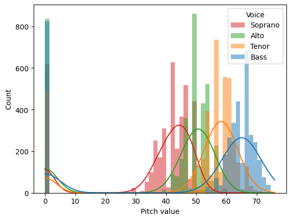
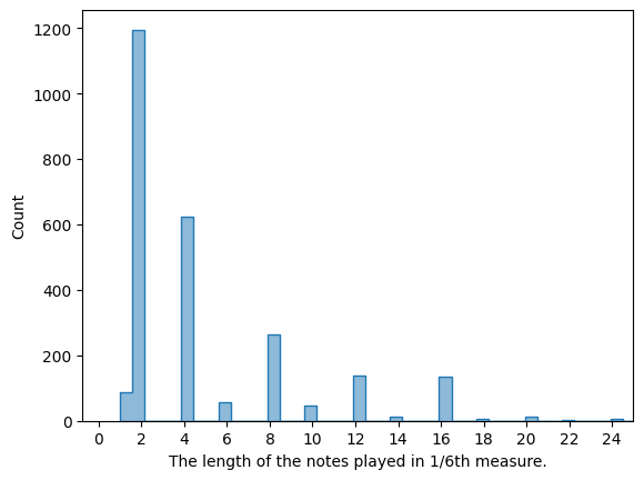
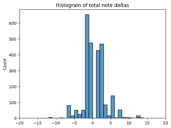
The charts show why the representation matters. Each voice occupies a distinct pitch range, and notes typically last 4 to 8 timesteps, not one. The encoding gives the model a head start on both facts.
Constrained sampling. The model outputs a softmax over all possible notes. Taking the argmax at every step produces exactly the kind of degenerate output the original project suffered from: the model locks onto a narrow set of notes and repeats them. The NoteSampler applies several constraints learned from the training data: a mask that restricts each voice to its observed pitch range, a frequency prior that biases toward common notes, a beat-position probability that encourages new notes at metrically strong positions, an interval constraint that penalizes jumps larger than those seen in the training data, and a chord quality scorer that compares the three intervals between the four voices against the distribution observed in Bach. At each generation step, 20 candidate combinations are drawn, scored, and the best one is selected.
The sampler does not guarantee good output. But it prevents the model from drifting into degenerate regions by anchoring the autoregressive loop to statistics that are known to be musical. It is a handrail, not a composer.
Training infrastructure. The pipeline has a proper CLI with all hyperparameters exposed as flags. A Config dataclass holds the defaults. Training uses ModelCheckpoint, EarlyStopping, ReduceLROnPlateau, and TensorBoard with histogram logging. At the end, the best checkpoint is loaded for generation. An evaluation harness compares the LSTM and Transformer side by side on test loss, accuracy, parameter count, inference time, and model size, and writes a JSON report. A grid search script sweeps over window size, dropout, filter counts, optimizer choice, and learning rate. All of this runs from the command line with no notebook required.
What I’d do differently
When we started this project in 2022, music generation was a niche subfield. There was no blueprint for a small model that produced coherent four-part harmony from a text file. You started from scratch or you did not start.
That has changed. In the years since, music generation has become a busy research area with established frameworks, benchmark datasets, and shared representations. If I were starting this project today, I would not begin with a five-dimensional hand-crafted encoding. I would use a mel spectrogram or a learned embedding trained on a larger corpus, then fine-tune on the Bach dataset. Representations that capture timbre, harmony, and rhythm simultaneously have become standard, and they outperform engineered features by a wide margin on most tasks. The lesson from this project is that representation is most of the work. Starting with a proven one would let me spend my time on the model behavior I actually want to study.
I would set up evaluation before writing the first line of model code. A listening test protocol, even an informal one with a few friends, would have caught the silence problem, the repetition problem, and the staccato duration problem within hours instead of weeks. A script that generates audio and plays it automatically after each training run would have turned subjective impressions into a rapid feedback loop. Right now the pipeline can output MIDI but the step from training to listening is still manual. Closing that loop is more valuable than shaving points off the loss.
I would not train four separate models again. The unified model predicting all voices at once was a clear improvement, but it was an obvious fix in hindsight. At the time, the four-model approach seemed simpler because each voice is a different instrument with a different range. But polyphony is fundamentally about the relationships between voices. Separating them at the architecture level removes the one thing that makes the problem interesting.
The end goal has not changed. I still want to find the smallest model that produces something melodic, and I still plan to run ablation experiments to see which parts actually matter. The difference is that I now know which parts of the problem are hard for reasons I did not anticipate, and which parts are hard because I made them harder than they needed to be.